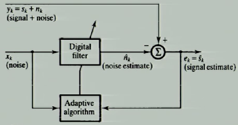
I watched a well organized and concise YouTube video about adaptive filters, which is the focus of an important course I am taking this semester, Digital Signal Processing II.
Limitations of fixed-coefficient digital filters
- Fixed-coefficient digital filters
- FIR, IIR
- LP, HP, etc
- Limitations
- Time-varying noise-frequency
- Overlapping bands of signal and noise
Adaptive filters

- 2 main components
- Digital filter (with adjustable coefficients)
- Adaptive algorithm
- 2 input signals: $y_k$ and $x_k$
- $y_k = s_k + n_k$
- $s_k$ = desired signal
- $n_k$ = noise
- $x_k$ = contaminating signal which is correlated with $n_k$, gives an estimate of $n_k$, i.e. $\hat{n_k}$
- Goal: produce optimum $\hat{n_k}$
- $e_k = \hat{s_k} = y_k - \hat{n_k} = s_k + n_k - \hat{n_k}$
- Theorem: minimize $e_k$, maximize the signal-to-noise ratio
LMS algorithm
Wiener filter

- An input signal w(n) is convolved w ith the Wiener filter g(n) and the result is compared to a reference signal s(n) to obtain the filtering error e(n)
- Criterion: MMSE (Minimum Mean Square Error)
- Minimize $J = E[e(n)^2] = E[(x(n) - s(n))^2] = E[(w(n) * g(n) - s(n))^2]$
- J can be used to draw the Error-Performance surface
- The Least mean squares filter converges to the Wiener filter
Wiener-Hopf solution
Set gradient of J of H to zero, deduced that
$H_{opt} = R_{xx}^{-1} R_{xs}$
where
$R_{xx} = E(X_k X_k^T)$
$R_{xs} = E(y_k X_k)$
- Requires knowledge of $R_{xx}, R_{xs}$
- Matrix inversion is expensive
- For non-stationary, $H_{opt}$ needs to be computed repeatedly
LMS adaptive algorithm
Version 1: $H(n+1) = H(n) + \mu (- \nabla(n))$
Version 2: $H(n+1) = H(n) + \frac{1}{2}\delta (- \nabla(n))$
then
$H(n+1) = H(n) + 2\mu e(n)X(n)$
or $H(n+1) = H(n) + \delta e(n)X(n)$
where
$e(n) = y(n) - H^T(n)X(n)$
$\mu$ and $\delta$ are step-sizes
- Based on the steepest descent algorithm (update H(n) along the opposite direction of the gradient):
$H(n+1) = H(n) + \mu (- \nabla(n))$ - Using instantaneous estimates instead of the means (unbiased):
$J = E[e(n)^2] = e(n)^2$
$\nabla(n) = -2\mu E[e(n)X(n)] = -2\mu e(n)X(n)$ - Step-size determines stablility and rate of convergence
- If too large, too much fluctuation
- If too small, convergences too slow
Limitations
- If the noise is non-stationary, the error-performance surface will change rapidly
- If $x(n)$ is proportional to $y(n)$, signal will be obliterated
- H(n) never reached the theoretical optimum (fluctuation)
Applications
- Acoustic echo cancellation
- Cancelling EOG from contaminated EEG and get correct EEG
- Cancelling maternal ECG and get foetal ECG during labour
Appendix
YouTube Video
Course Home Page
Comments